Médecine Sciences
Physique pour l'imagerie
Benoît C. FORGET
2016-17
Laboratoire neurophotonique
Faculté des Scicences Fondamentales et Biomédicales
benoit.forget@parisdescartes.fr

Plan
- Rappels d'optique géométrique
- Rayons et Images
- Microscope Optique
- Notion d'onde
- Propagation d'onde
- Description mathématique des ondes
- Équation de d'Alembert
- Solutions harmoniques
- Notation complexe
- Dualité temps fréquence
- Rayons et Images
- Microscope Optique
- Propagation d'onde
- Description mathématique des ondes
- Équation de d'Alembert
- Solutions harmoniques
- Notation complexe
- Interférences et Diffraction
- Imagerie de phase
- Résolution et PSF
- PSF et convolution
- Super résolution
- Wavefront Engineering
- Ondes à 2 et 3 dimensions : Notion de front d'onde
- De l'optique ondulatoire à l'optique géométrique
- Applications aux neurosciences
- Absorption
- Oscillateur harmonique : modèle universel
- Polarisation
- Exemple : spectre d'absorption de l'eau
- Imagerie de phase
- Résolution et PSF
- PSF et convolution
- Super résolution
- Ondes à 2 et 3 dimensions : Notion de front d'onde
- De l'optique ondulatoire à l'optique géométrique
- Applications aux neurosciences
- Oscillateur harmonique : modèle universel
- Polarisation
- Exemple : spectre d'absorption de l'eau
Propagation de la lumière et formation d'images
Trois modèles pour l'optique
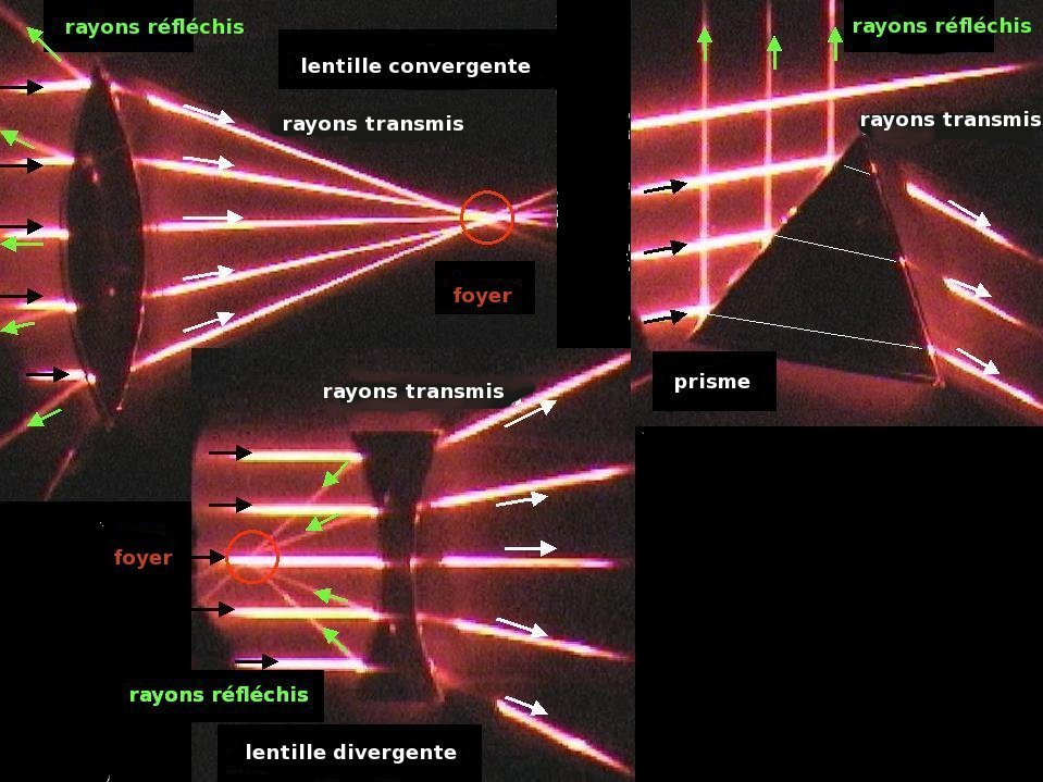
- L'optique géométrique
- "rayon lumineux" pour étudier la propagation de la lumière et la formation d'images ;
- "lois empiriques" de propagation rectiligne, de réflexion et réfraction ;
- permet la conception d'instruments (eg. télescope, microscope, fibres optiques ...)
- L'optique ondulatoire
- Modèle scalaire
- décrit les interférences, la diffraction, la diffusion, etc. ;
- applications : mesures interférométrique (très haute précision) et la spectroscopie
- Ondes électromagnétiques
- notion de polarisation
- L'optique quantique
- émission de la lumière et interaction avec les atomes, les molécules ;
- a permis en particulier le développement du laser.
Optique géométrique
- rayon lumineux pour étudier la propagation de la lumière et la formation d'images ;
- lois empiriques de propagation rectiligne, de réflexion et réfraction ;
- permet la conception d'instruments (eg. télescope, microscope, fibres optiques ...)
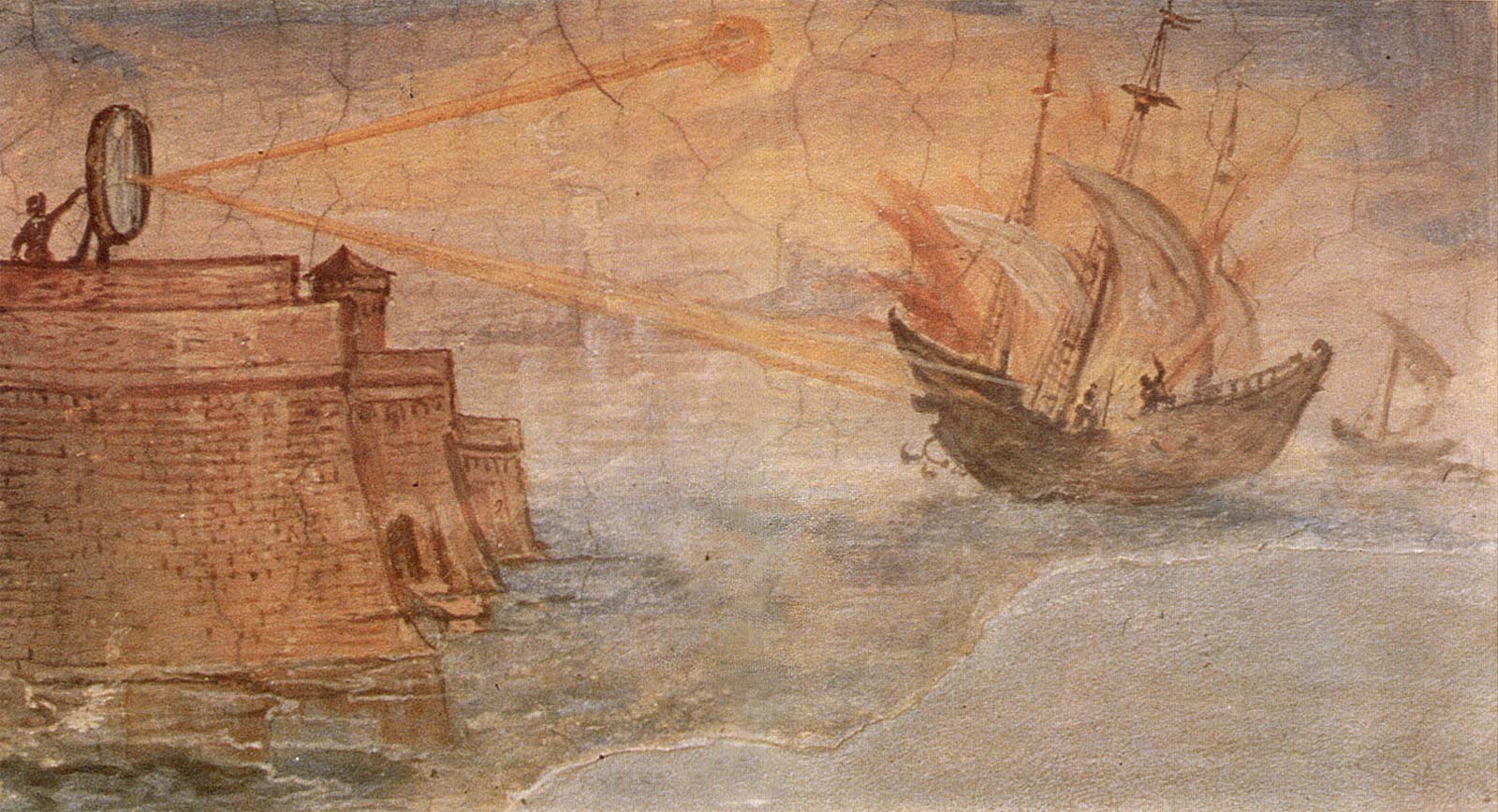
Wall painting from the Stanzino delle Matematiche in the Galleria degli Uffizi (Florence, Italy). Painted by Giulio Parigi (1571-1635) in the years 1599-1600.
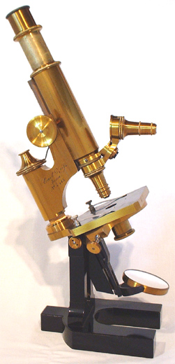
Microscope Zeiss, circa 1879, d'autres de la même époque ici : Museum optischer Instrumente
Stigmatisme et Formation d'Images
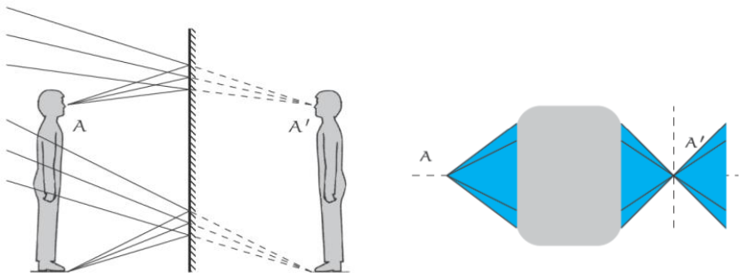
- le système est stigmatique pour les points \(A\) et \(A'\) ;
- \(A'\) est le point conjugué du point \(A\) : \(A'\) est l'image \(A\) ;
- tout rayon lumineux dont le support dans le milieu incident passe par \(A'\) a son support dans le milieu émergeant passant par \(A'\) ;
- en l'absence de stigmatisme, l'image est floue
image nette
Is there a bijective relation between "object" and "image" : can we recover the "object" from the "image" ?
Dioptres
Reflection et Refraction : A at the interface between two media of different index of refraction a ray of light changes it's direction.
Lois de Snell - Descartes
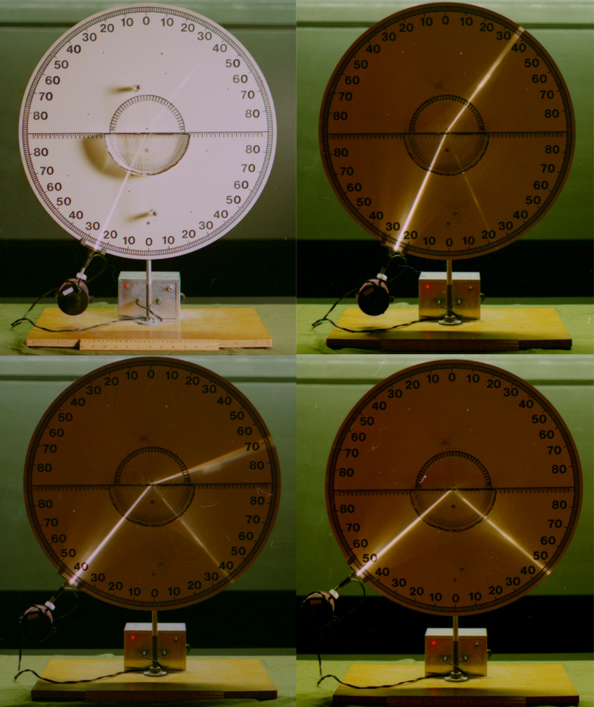
- Réflexion : $$ i = -r $$
- Réfraction : $$ n_1 \sin i_1 = n_2 \sin i_2 $$
- Conditions de Gauss : $$ \sin i \approx i $$
- Retour inverse de la lumière
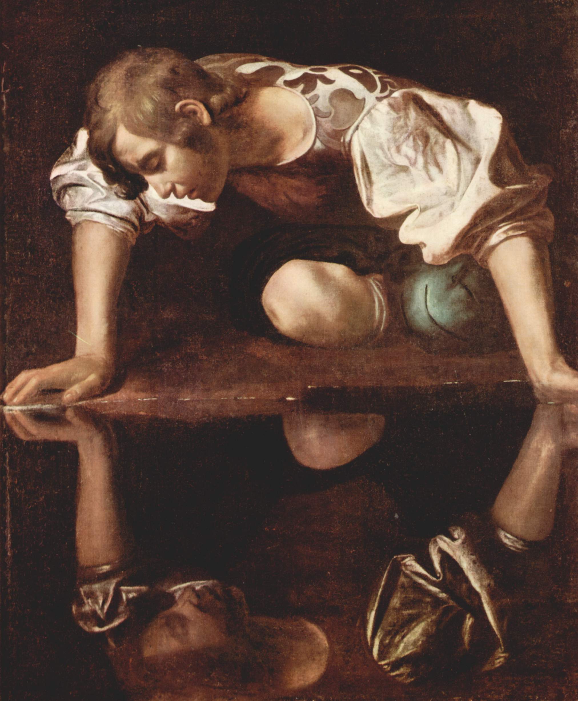
Mais qui regarde Venus ?
Véronese 1585 : Vénus au miroir
Lentilles minces
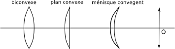
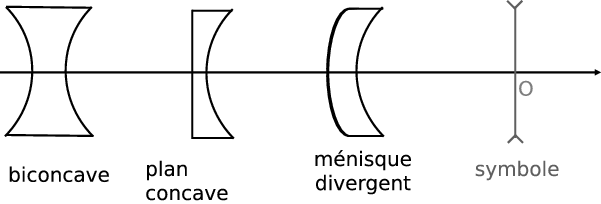
Relation de conjugaison
$$ \frac{1}{\overline{OA'}}-\frac{1}{\overline{OA}}=\frac{1}{\overline{OF'}} \left(=-\frac{1}{\overline{OF}} \right) $$Points (et plans) focaux
Le point focal est conjugué avec l'infini
Les systèmes complexes peuvent aussi être décrit par leurs foyers (et plans conjugués)
Grandissement (transverse)
$$ \gamma_t = \frac{\overline{A'B'}}{\overline{AB}}=\frac{\overline{OA'}}{\overline{OA}}$$Système afocal
Loupe, grossissement (angulaire)
Qu'est-ce qu'un microscope ?
Instrument qui:
- donne une image grossie d’un petit objet (grossissement)
- sépare les détails de celui-ci sur l’image (résolution)
- rend les détails visibles à l’œil ou avec une caméra
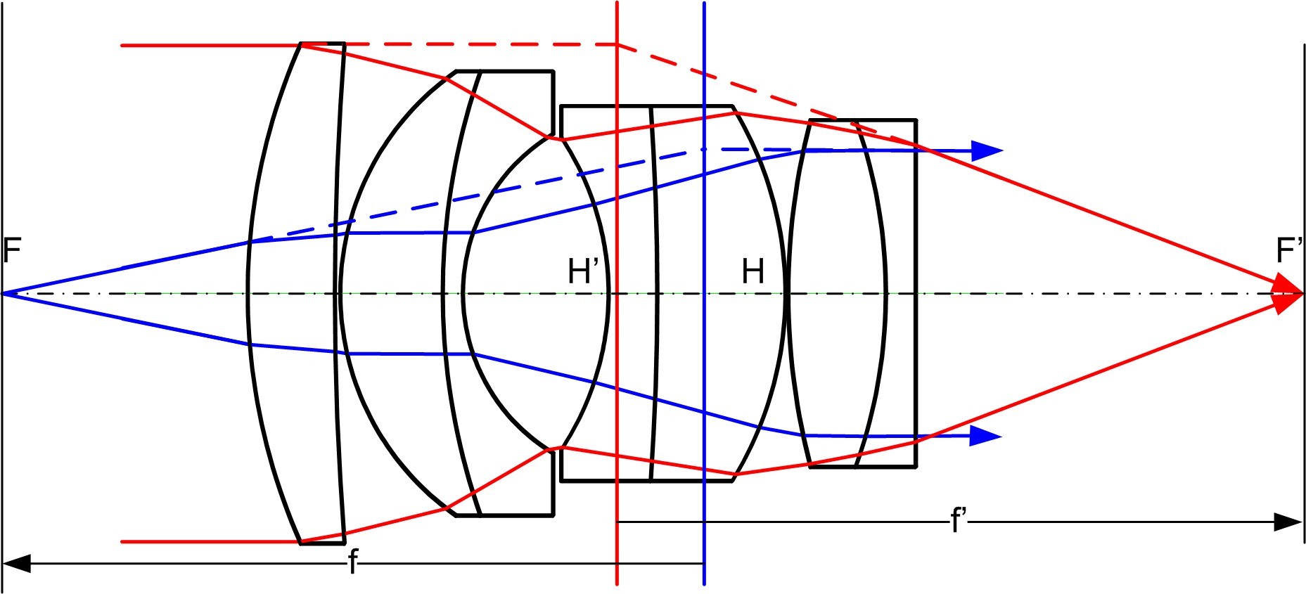
Objectif

Site de référence sur la microscopie :
Perfect Two-Lens System
![]()
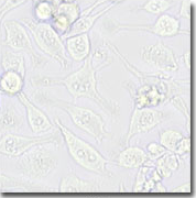
Le grossissement ne suffit pas !
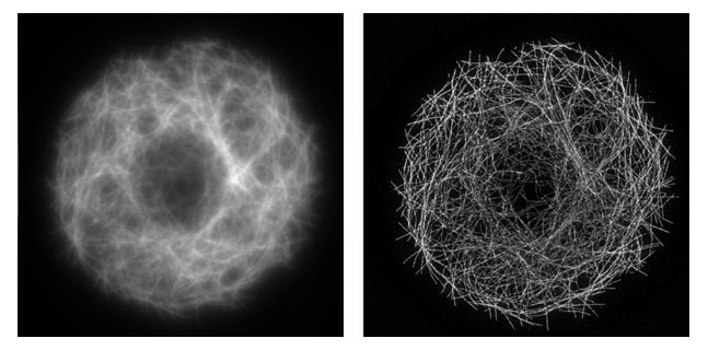
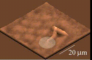
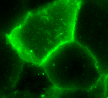
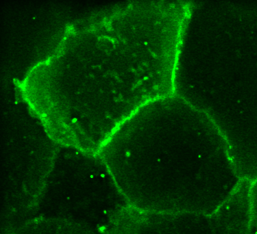
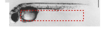
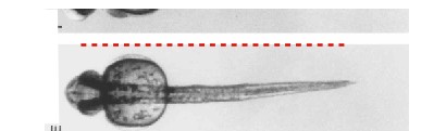
Microtubules de cellules S2 de drosophile
Optique ondulatoire
Qu'est-ce qu'une onde ?
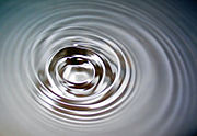
Dans un milieu élastique il existe des forces internes qui tendent à le ramener à sa situation d'équilibre après une perturbation
Cette perturbation (ou déformation) se déplace à une vitesse (célérité) qui est déterminée uniquement par les propriétés mécaniques de ce milieu.
A deformation moving while keeping the same shape
Space and time evolution (variables) are 'coupled':
Is there an equation that allows for solution :
$$A\xi(x-ct)+B\xi(x+ct)$$
d'Alembert equation !
$$\frac{\partial^2 \xi}{\partial t^2} - c^2 \frac{\partial^2 \xi}{\partial x^2} =0 $$
Analyse dimensionnelle :
$$ \frac{[\xi]}{[T]^2}-[c]^2\frac{[\xi]}{[L]^2} \;\to\; [c]=\frac{[L]}{[T]}$$
La célérité \(c\) a bien les dimensions d'une vitesse.
Newtonian dynamics ... \(\displaystyle \to\quad \frac{\partial^2 \xi}{\partial t^2}-c^2\frac{\partial^2 \xi}{\partial x^2}=0\)
Si les angles sont petits : \(\displaystyle \sin \theta_{1,2} \approx \tan\theta_{1,2} = \left.\frac{\partial \xi} {\partial z}\right| _{z=z_1,z=z_2}\)
et si la corde ne se déforme pas : \(\displaystyle T_2 \approx T_1 \equiv T_0 \)
et donc : \(\displaystyle F_x(t)= T_0 \left.\frac{\partial \xi}{\partial z}\right|_{z=z_2} -T_0 \left.\frac{\partial \xi}{\partial z}\right|_{z=z_1}= T_0 \Delta z \frac{\partial^2 \xi}{\partial z^2}\)
Il faut d'appliquer la seconde loi de Newton : \(\vec F = m\vec a\).
$$ \xi\to\textrm{déplacement}\; ;\; \frac{\partial \xi}{\partial t}\to\underbrace{\textrm{vitesse}}_{\neq \textrm{célérité !}} \; ;\; \frac{\partial^2 \xi}{\partial t^2}\to \textrm{accélération} $$
La masse linéïque (masse par unité de longueur) \(\rho\) permet d'exprimer la masse \(m\) du segment : \(m=\rho\Delta z\)
$$F_x(t)= ma \to T_0 \Delta z \frac{\partial^2 \xi}{\partial z^2} = \rho \Delta z \frac{\partial^2 \xi}{\partial t^2} \;\to\; \frac{\partial^2 \xi}{\partial z^2} - \frac{\rho}{T_0} \frac{\partial^2 \xi}{\partial t^2} =0$$
Newtonian dynamics + fluid elasticity ... \(\displaystyle \to\quad \frac{\partial^2 p}{\partial t^2}-c^2\frac{\partial^2 p}{\partial x^2}=0\)
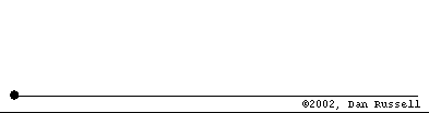
La déformation \(\xi\) est fonction du temps \(t\) et de la position \(x\), de la forme : \(\xi(x,t) = f(x-ct)\).
$$ F=ma \quad\to\quad S
\underbrace{\left[p(x) - p(x+\Delta x) \right]}_{=-\frac{\partial p}{\partial x} \Delta x}
= \rho S \Delta x \frac{\partial^2\xi}{\partial t^2} $$
\[ -\frac{\partial p}{\partial x} = \rho \frac{\partial^2\xi}{\partial t^2} \quad\to\quad \frac{\partial p}{\partial x} + \rho \frac{\partial^2\xi}{\partial t^2} = 0\]
\[ \rho V = \rho_0 V_0 \;\to\; \frac{\rho}{\rho_0} = \frac{V_0}{V} = \frac{S\Delta x}{S\Delta x \left[1+\frac{\partial \xi}{\partial x} \right]} \]
\[ \frac{\rho}{\rho_0} = \frac{1}{1+\frac{\partial \xi}{\partial x} } = 1-\frac{\partial \xi}{\partial x} \;\to\; -\frac{\partial \xi}{\partial x} = \frac{\rho-\rho_0}{\rho_0} = \frac{\Delta\rho}{\rho_0} \]
ou
\[ \frac{V}{V_0} = 1+\frac{\partial \xi}{\partial x} \;\to\; \frac{\partial \xi}{\partial x} = \frac{V-V_0}{V_0} = \frac{\Delta V}{V_0} \]
La description qui prend en compte la géométrie 3D relie linéairement la pression à la variation relative de volume :
$$ p = cste \cdot \frac{\Delta V}{V_0} \;\to\; p = -\frac{1}{\chi} \frac{\Delta V}{V_0} \;\to\; \frac{\Delta V}{V_0} = -\chi p $$
Dans le cas qui nous intéresse, \(\chi\) est la compressibilité adiabatique.
\begin{align*}
\frac{\partial p}{\partial x} + \rho \frac{\partial^2\xi}{\partial t^2} = 0 & \\
\frac{\partial}{\partial x}\left[-\frac{1}{\chi}\frac{\Delta V}{V_0} \right] + \rho \frac{\partial^2\xi}{\partial t^2} = 0 & \\
-\frac{1}{\chi}\frac{\partial}{\partial x}\left[ \frac{\partial \xi}{\partial x}\right] + \rho \frac{\partial^2\xi}{\partial t^2} = 0 & \to \frac{\partial^2\xi}{\partial t^2} -\frac{1}{\chi\rho}\frac{\partial^2 \xi}{\partial x^2} = 0\\
\end{align*}
Note that vacuum (like materials) has electromagnetic properties !
Trig functions (sine, cosine) are solution to d'Alembert's equation.
In the form :
$$\xi(x,t)= A\cos(kx \pm \omega t+ \phi ) $$
with : \(\displaystyle c=\frac{\omega}{k}\)
Vérification :
\begin{align*}
\frac{\partial}{\partial t}\left[ \frac{\partial }{\partial t} A \cos(\omega t - kx + \varphi) \right]
- c^2\frac{\partial}{\partial x}\left[\frac{\partial }{\partial x}A\cos(\omega t - kx + \varphi)\right] &= 0 \\
\frac{\partial}{\partial t}\left[-\omega A\sin(\omega t - kx + \varphi)\right] - c^2\frac{\partial}{\partial x}\left[kA\sin(\omega t - kx + \varphi)\right] &= 0 \\
-\omega^2 A\cos(\omega t - kx + \varphi) + c^2k^2A\cos(\omega t - kx + \varphi) &= 0
\;\to\; c=\frac{\omega}{k}
\end{align*}
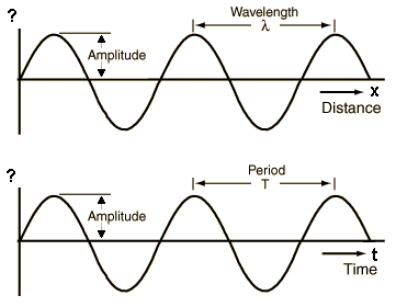
Space (\(\lambda\)) and time (\(T\)) periodicity are explicited :
$$\cos\left(2\pi\left(\frac{x}{\lambda} \pm \frac{t}{T}\right)+ \phi \right )$$
$$k=\frac{2\pi}{\lambda} \; ; \; \omega = 2\pi f = \frac{2\pi}{T} \quad\to \quad c=f\lambda$$
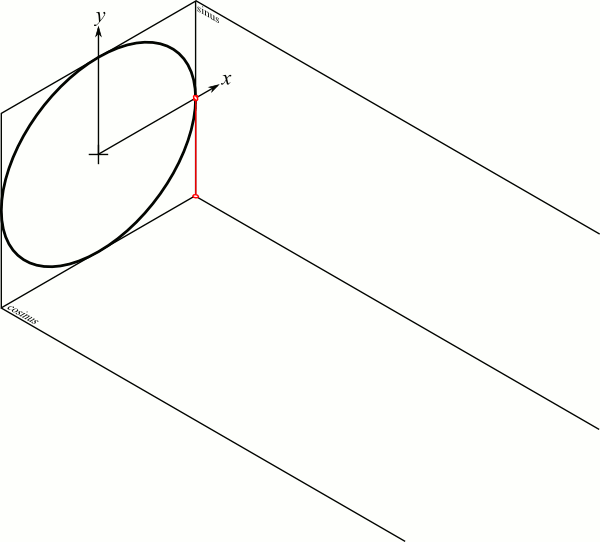
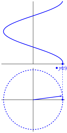
Avant de pousser plus loin, considérons un mouvement circulaire uniforme
donc :
$$ \theta =\omega t + \theta_0$$
\(\omega\) est la vitesse angulaire et \(\theta_0\) l'angle initial (en \(t=0\))
En coordonnées cartésiennes :
$$ \vec x= \ell \cos\theta \vec u_x \qquad \vec y=\ell\sin\theta \vec u_y \quad \left[=\ell\sin\left(\theta -\frac{\pi}{2}\right)\vec u_y\right]$$
On peut repérer la position (\(\overrightarrow{OA}\)) comme suit :
On s'intéresse maintenant à la vitesse :
$$\vec v= \frac{d\overrightarrow{OA}}{dt} = \ell \frac{d}{dt} \left[\cos\left(\omega t + \theta_0\right) \vec u_x + \sin\left(\omega t + \theta_0\right) \vec u_y \right] $$
\begin{align*}
\vec v &= \omega\ell \left[-\sin\left(\omega t + \theta_0\right) \vec u_x + \cos\left(\omega t + \theta_0\right) \vec u_y \right] \\
& = \omega\ell \left[-\sin\theta \vec u_x + \cos\theta \vec u_y \right] = \omega\ell \vec u_t
\end{align*}
La vitesse est tangentielle :
$$\vec v= \omega\ell \left[-\sin\theta \vec u_x + \cos\theta \vec u_y \right]= \omega\ell \vec u_t$$
La vitesse varie en fonction du temps, on s'intéresse maintenant à l'accélération :
\begin{align*}
\vec a & = \frac{d\vec v}{dt} \\
& = \omega\ell \frac{d}{dt} \left[-\sin\left(\omega t + \theta_0\right)\vec u_x + \cos\left(\omega t + \theta_0\right) \vec u_y \right] \\
&=\omega^2\ell \vec u_c
\end{align*}
avec \( \vec u_c = -\cos\theta \vec u_x - \sin\theta \vec u_y = -\vec u\) ! L'accélération est bien centripète.
Il y a deux façons de repérer le point \(A\) :
$$ x=a\cos\theta \; ; \; y=a\sin\theta $$
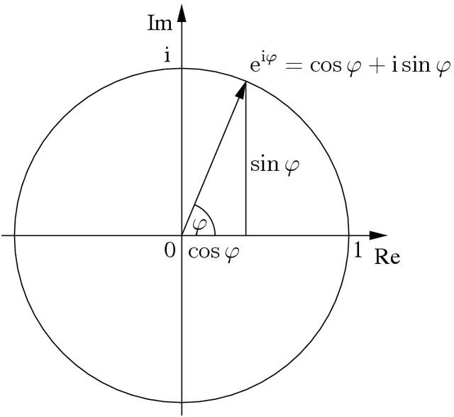
On choisira de représenter la position \(A\) par un nombre complexe
Avantage de l'exponentielle complexe :
$$ z=ae^{i\theta} \quad\to\quad \frac{\partial z}{\partial \theta} = iae^{i\theta} = iz $$
la dérivée s'obtient par une multiplication.
Position :
$$ A=\ell e^{i\omega t}$$
Vitesse :
$$ \frac{\partial A}{\partial t} = i\omega \ell e^{i\omega t}$$
Accélération :
$$ \frac{\partial^2 A}{\partial t^2} = (i\omega)^2 \ell e^{i\omega t} = -\omega^2\ell e^{i\omega t}$$
$$\frac{\partial }{\partial t} = \times i\omega$$
\begin{align*}
i &= e^{i\frac{\pi}{2}}=\cos\frac{\pi}{2}+i\sin\frac{\pi}{2} = 0 +i1 =i \\
i^2 &= e^{i\pi} =-1 \\
i^3 &= e^{i\frac{3\pi}{2}} = -i \\
...
\end{align*}
The EM field \(E(x,t)\)is written in complex notation :
\begin{align*}
E=A\cos(kx \pm \omega t + \phi) & = \Re\left\{\tilde E = Ae ^{j(kx \pm \omega t + \phi)}\right\} \\
& = \Re\left\{\tilde E = Ae ^{j\phi}e ^{j(kx \pm \omega t)}\right\} \\
& = \Re\left\{\tilde E =\tilde Ae ^{j(kx \pm \omega t)}\right\}
\end{align*}
Note: Physical (measurable) quantites can only be expressed with real numbers.
Cette approche fonctionne tant que l'on s'en tient à des opérations linéaires :
$$\Re\{ a z_1 + z_2\} = a \Re z_1 + \Re z_2 $$
$$ \Re\{ z'\} = (\Re z )' $$
mais :
$$\Re\{ z_1 \times z_2\} \neq \Re z_1 \times \Re z_2 $$
For example, a sound wave :
$$f=1000\,{\rm Hz} \; ;\; c=330\,{\rm m.s^{-1}} \quad\to\; \lambda = 0,33\,\textrm{m}$$
One particular "point" of phase \(\varphi_0\) travels along the axis \(Ox\) at speed \(c\).
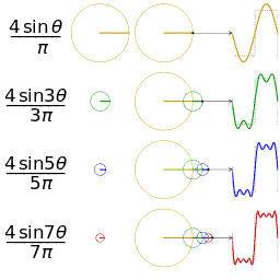
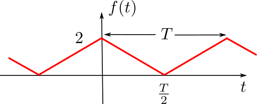
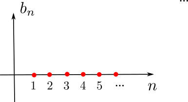
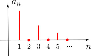
Toute fonction périodique \(f(t)\) de période \(T\) (de pulsation \(\omega\), \(\omega T=2\pi\)) peut s'écrire comme suit :
\begin{align*}
f(t) &= a_0 + a_1\sin\omega t + b_1 \cos\omega t + a_2\sin 2\omega t + b_2 \cos 2\omega t + \ldots \\
&= a_0 + \sum_n a_n \sin n\omega t + \sum_n b_n \cos n\omega t
\end{align*}
Il suffit de savoir calculer les coefficients :
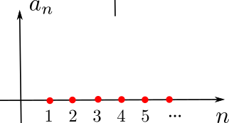
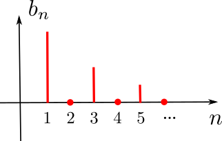
Remarquez l'effet de la parité de la fonction !
Formule d'Euler :
\begin{align*}
f(t) &= a_0 + \sum_n a_n \sin n\omega t + \sum_n b_n \cos n\omega t \\
&= a_0 + \sum_n a_n \frac{e^{in\omega t}-e^{-in\omega t}}{2i} + b_n \frac{e^{in\omega t}+e^{-in\omega t}}{2} \\
&= a_0 + \sum_n \frac{b_n-ia_n}{2}e^{in\omega t} + \frac{b_n+ia_n}{2}e^{-in\omega t} \\
&= a_0 + \sum_n c_n e^{in\omega t} + c_n^* e^{-in\omega t}
\end{align*}
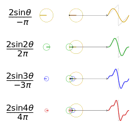
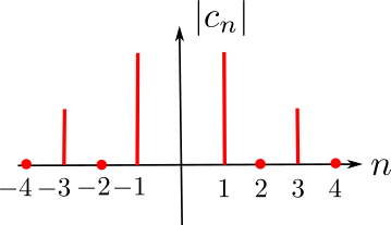
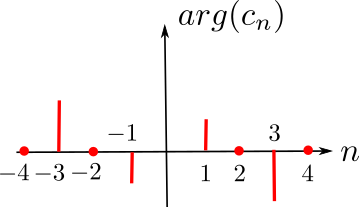
Série complexe, fréquences "négatives"
$$f(t)=\sum_{n=-\infty}^{\infty} c_n e^{in\omega t} \quad ;\; c_n=\frac{1}{T}\int_0^T f(t) e^{-in\omega t}dt \quad ;\; c_n^* = c_{-n} $$
On définit la transformée de Fourier (TF), notée \(X(f)\), d'un signal \(x(t)\) et son inverse comme suit :
\[ TF\{x(t)\} \equiv X(f) = \int_{-\infty}^\infty x(t)e^{-j2\pi ft} dt\]
\[ TF^{-1}\{X(f)\} \equiv x(t) = \int_{-\infty}^\infty X(f)e^{+j2\pi ft} df\]
$$
\left. \begin{array}{ll}
1\,\textrm{battement :} & 1,2\,\textrm{sec.} \\
6\,\textrm{battements :} & 7,1\,\textrm{sec.}
\end{array}
\right\} \;\to\; 50,7\,\textrm{bat/min} \;\to\; 0,83 \textrm{Hz}
$$
Remember that d'Alembert's equation is linear : the sum of fundamental solutions (monochromatic waves) is also a solution (polychromatic wave)
Acoustic beats is the simplest example :
Transport d'énergie sans transport de matière
Mathematical description of waves
$$\xi(x,t) = \xi(x-ct) \qquad\left\{\xi(x+ct)\;\textrm{if}\; \vec c= -c \vec u_x \right\}$$
From a mathematical point of view
From a physical point of view
Vibrating string
From a physical point of view
pressure wave in a sound pipe
Démonstration : Dynamique
On définit :
Conservation de la masse
$$ V_0 = S \Delta x $$
\begin{align*}
V &= S\left[ \Delta x + \xi(x+\Delta x) - \xi(x)\right] \\ &= S\Delta x\left[1+\frac{\partial \xi}{\partial x}\right]
\end{align*}
Élasticité : Loi de Hooke
$$F=k\Delta \ell$$
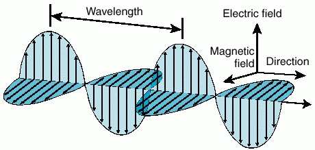
What about EM waves ?
 \begin{align}
\vec \nabla \cdot \vec E &= \frac{\rho}{\varepsilon_0} \\
\vec \nabla \cdot \vec B &= 0 \\
\vec \nabla \times \vec E &= -\frac{\partial\vec B}{\partial t} \\
\vec \nabla \times \vec B &= \mu_0 \vec j + \mu_0\varepsilon_0\frac{\partial\vec E}{\partial t} \\
\end{align}
$$-\nabla^2 \vec E +\mu_0\varepsilon_0 \frac{\partial^2 \vec E}{\partial t^2} = 0$$
$$ c=\frac{1}{\sqrt{\mu_0\varepsilon_0}} $$
\begin{align}
\vec \nabla \cdot \vec E &= \frac{\rho}{\varepsilon_0} \\
\vec \nabla \cdot \vec B &= 0 \\
\vec \nabla \times \vec E &= -\frac{\partial\vec B}{\partial t} \\
\vec \nabla \times \vec B &= \mu_0 \vec j + \mu_0\varepsilon_0\frac{\partial\vec E}{\partial t} \\
\end{align}
$$-\nabla^2 \vec E +\mu_0\varepsilon_0 \frac{\partial^2 \vec E}{\partial t^2} = 0$$
$$ c=\frac{1}{\sqrt{\mu_0\varepsilon_0}} $$
trig functions as solutions

Digression : Notation complexe

Vitesse tangentielle

$$ \overrightarrow{OA} = \ell \cos\theta \vec u_x + \ell\sin\theta \vec u_y = \ell \vec u $$
avec \(\vec u = \cos\theta \vec u_x + \sin\theta \vec u_y\).
avec \(\vec u_t=-\sin\theta \vec u_x + \cos\theta \vec u_y\).
\(\vec u_t\) est perpendiculaire à \(\vec u\).
Accélération centripète

Représentation complexe

$$a= \sqrt{x^2+y^2} \; ;\; \theta=\textrm{atan}\frac{y}{x}$$
Représentation cartésienne, Représentation polaire
$$ z= x+iy \quad\textrm{avec}\, i=\sqrt{-1} $$
 $$ z= a\underbrace{\left(\cos\theta+i\sin\theta)\right)}_{=\exp(i\theta)\,\textrm{: rel. d'Euler}} = ae^{i\theta} $$
Dérivée

multiplication par \(i\)
$$z_1=a_1e^{i\theta_1}\; ;\; z_2=a_2e^{i\theta_2} \quad\to\quad z_4=z_1z_2=a_1a_2e^{i(\theta_1+\theta_2)}$$

Onde en notation complexe
Attention au caractère linéaire
The traveling wave
$$\tilde{E}=\tilde{A}e^{j( \omega t \pm kr)}$$
 https://commons.wikimedia.org/w/index.php?curid=31381808
Propagating wave : the phasor
\begin{align}
\omega t -kw &= \varphi_0 \\
x &= \frac{\varphi_0}{k}+\frac{\omega}{k}t \\
&= \frac{\varphi_0}{k}+ct
\end{align}
3. Dualité temps fréquence
Optical Waves
Séries et transformée de Fourier
C'est la valeur moyenne de \(f(t)\).
Espaces vectoriels, Espaces de Hilbert : Analogie
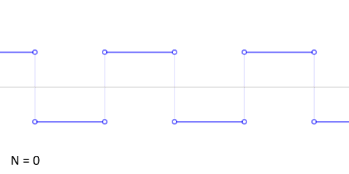
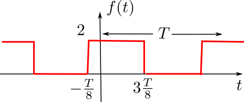
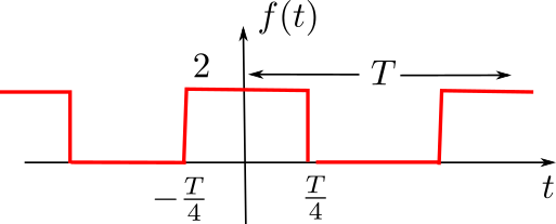
Signal "Carré"

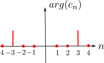
Représentation spectrale


en complexes
$$ e^{i\theta}=\cos\theta +i\sin\theta \quad\to\quad \cos\theta = \frac{e^{i\theta}+e^{-i\theta}}{2} \; ;\; \sin\theta = \frac{e^{i\theta}-e^{-i\theta}}{2i}$$

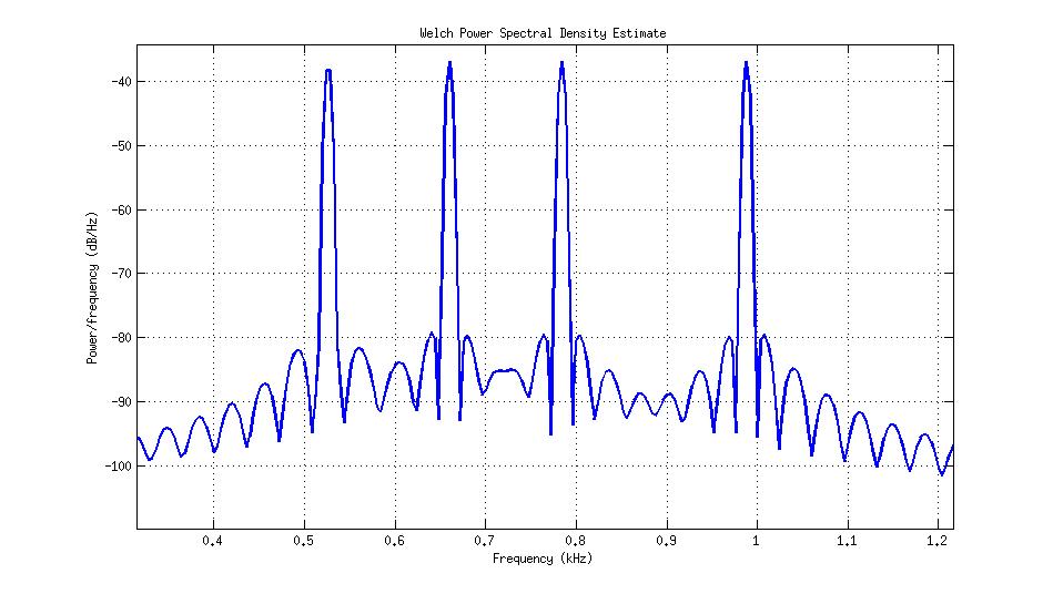
Transformée de Fourier
Notion d'analyse fréquentielle
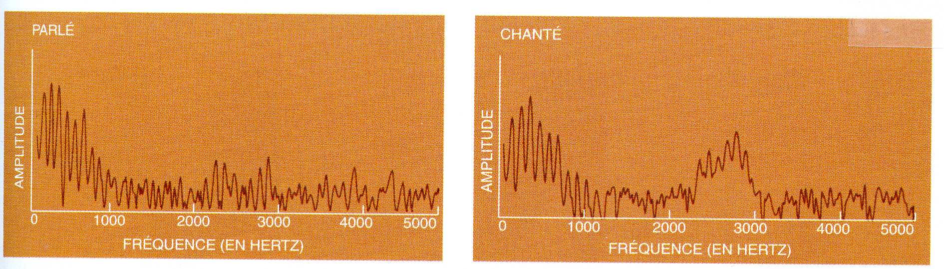
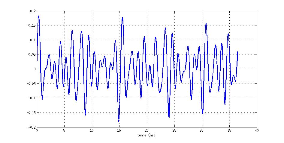
Exemple : ECG

Son musical
Analyse temps-fréquence

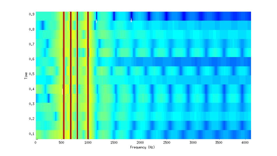
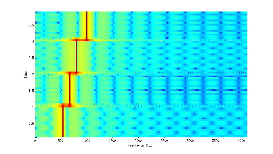
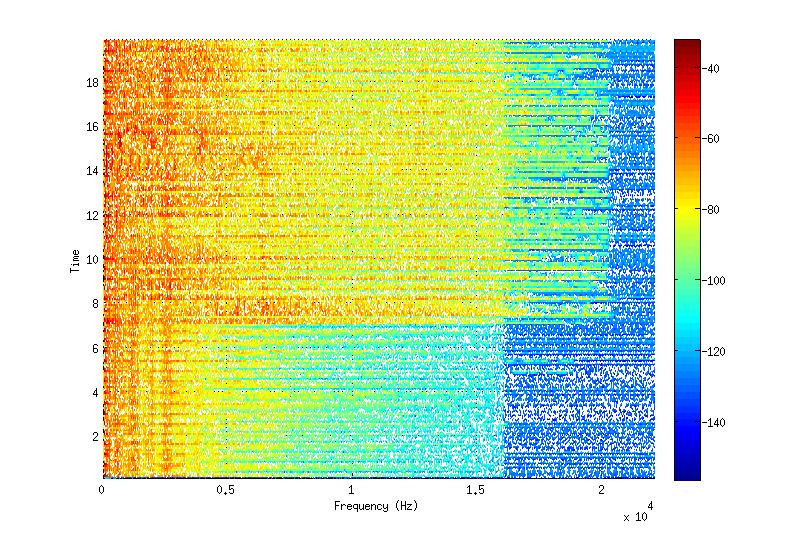
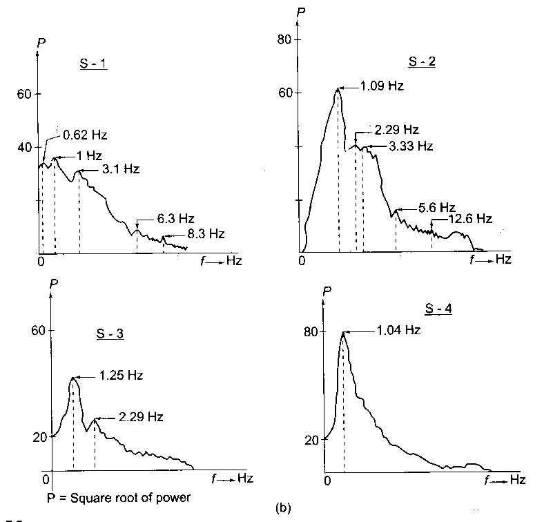
ECG : arythmie


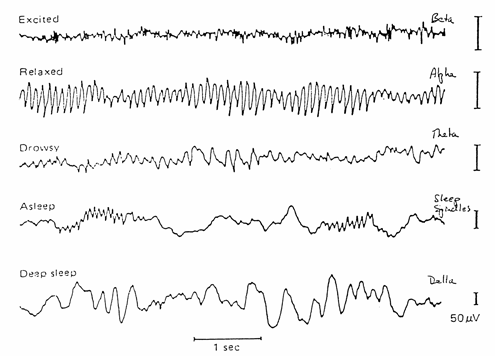
EEG : phases du sommeil
Transformée de Fourier 2D
Filtre passe-bas, Filtre passe-haut

Et la phase ?

Laser à impulsions brèves
Amplitude modulation
desafinado :
More waves ...
Why is this too easy ?
The solution to d'Alembert's equation implies a phase reference \(\varphi\) :
$$ A \exp\left(j\left(\omega t -k x + \color{orange}{\varphi}\right)\right)$$
This phase reference sets the "origin" of space and time.
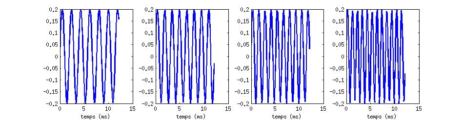
Remember mode locking
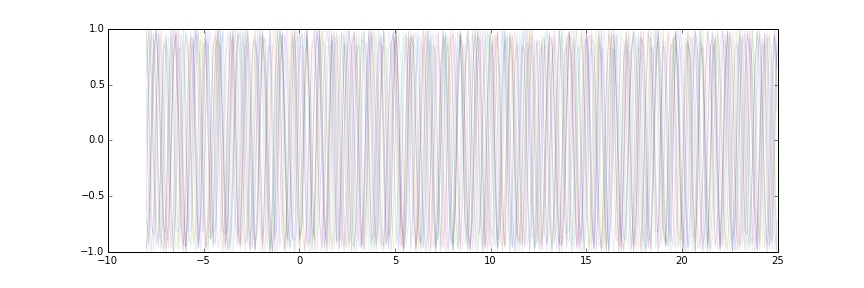
The simulations shown before are "mode locked". This means that \(\varphi\) is the same for every wave in the sum.
What if the phase is randomly distributed ?
frequency content

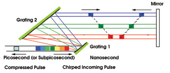
Compressing and Stretching chirped pulses
A dispersive device (grating, prism, ...) can seperate the frequencies (colors) contained in a short pulse.
4. Interférences et Diffraction
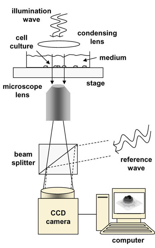
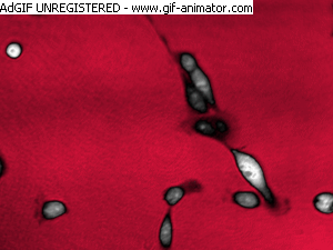
Seeing water in water
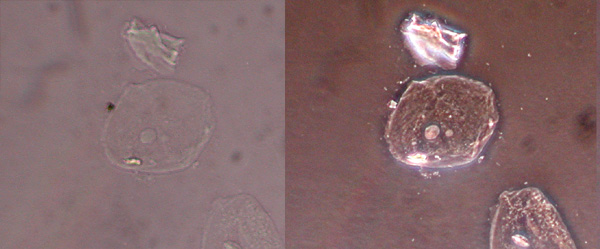
Intensity constrast
Brightfield reflectance microscopy is based on intensity constrast
$$ R=\frac{\left(n_1-n_2\right)^2}{\left(n_1+n_2\right)^2} $$
The cell is not verry "optically different" than the sourounding medium :
Cell : \(n = 1, 36 \,\to\, R\approx 0, 0233\)
nutriment medium : \(n = 1, 335 \,\to\, R \approx 0, 0206\)
Contrast : \( \displaystyle C=\frac{I_{max}-I_{min}}{I_{max}+I_{min}} \approx 6\% \)
Why not measure phase contrast
$$\Delta\varphi = k\Delta(nz) = \frac{2\pi}{\lambda}z\Delta n$$ $$z=6 µm\,;\, \Delta n =0,025 \,;\, \lambda=0,5 µm$$ $$\Delta (nz)=\frac{\lambda}{4}\,;\,\Delta\varphi \approx \frac{\pi}{2} $$
| detector | response time |
| eye | \( \approx 0,1\) s |
| photo film | \( \approx 10^{-4} - 10^{-2} \) s |
| electronic detector | \( \approx 10^{-6} - 10^{-2}\) s |
| CCD | \( \approx 10^{-2}\) s |
$$ c=3\times 10^8 {\rm m/s} $$ $$ 400 {\rm nm} < \lambda < 700 {\rm nm} $$ $$ f= 6\times 10^{14} {\rm Hz} $$
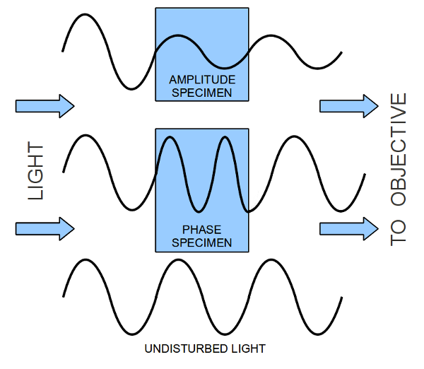
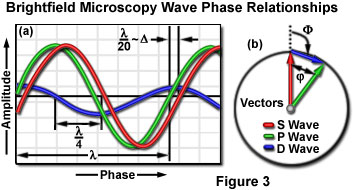
Amplitude, phase and intensity
Remember the expression of the field (in complex and real notations) : $$ \tilde E = \tilde A e^{j(kr - \omega t)} $$ $$ \Re\{E\} = A \cos (kr - \omega t + \varphi) $$
Only the intensity (average value over tile of the energy of the wave) can be detected. $$ I = \left < E^2 \right > = \frac{1}{2} EE^* = \frac{A^2}{2} $$
Detection of the intensity is phase independant !
Interferences
D'Alembert's equation is linear
The sum of the wave (interference) is also a wave : $$ E_1 = \tilde A e^{j(kr - \omega t)} \qquad E_2 = \tilde A e^{j(kr - \omega t+\Delta \phi)} $$
The intensity of this interference is phase dependant : $$ I_T = \frac{1}{2} (E_1+E_2)(E_1+E_2)^* = I_1+I_2+2\sqrt{I_1I_2}\cos \Delta\phi $$
it is a function of the phase difference \(\Delta \varphi\) between the two intefering waves.
A simple example : Young' slits
Why do we see (weak) contrast here ?
Where is the "second wave" ?
Abbe's theory of image formation
 $$ d=\frac{\lambda}{2n\sin \alpha}$$
An image is a spatial distribution of intensity, the intensity of the total field reaching the image plane
This total field can be expressed as the sum of individual fields and the image can "viewed" as the interference pattern genrated by these individual fileds !
Fourier series
Any periodic function \(f(t)\) of period \(T\) (pulsation \(\omega\), \(\omega T=2\pi\)) can be expressed as :
\begin{align*}
f(t) &= a_0 + a_1\sin\omega t + b_1 \cos\omega t + a_2\sin 2\omega t + b_2 \cos 2\omega t + \ldots \\\
&= a_0 + \sum_n a_n \sin n\omega t + \sum_n b_n \cos n\omega t
\end{align*}


Abbe's diffraction limit


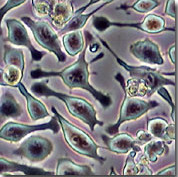
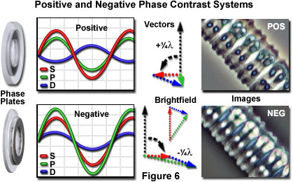
Phase contrast image
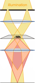
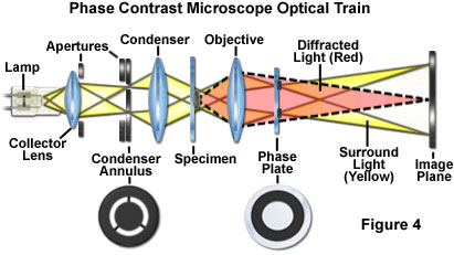
- "Some part" of the incoming wave interacts with the sample. This is the "diffracted wave"
- "Some other part" of the incoming just "goes right through". This is the "surrond wave".
- The image results from the interference between these two waves
Optimizing phase contrast
$$ I_T = I_1+I_2+2\sqrt{I_1I_2}\cos \Delta\phi $$$$ I_T \approx I_S+2\sqrt{I_SI_D}\cos \Delta\phi $$
$${\cal C} \equiv \frac{I_2-I_1}{I_2+I_2} \qquad\to\quad {\cal C} \propto 1- \cos\Delta\phi \approx \Delta\phi ^2 $$
Phase shift the surround wave
$$ I_T = I_1+I_2+2\sqrt{I_1I_2}\cos \Delta\phi $$$$ I_T \approx I_S+2\sqrt{I_SI_D}\cos (\Delta\phi +\pi/2) \approx I_S+2\sqrt{I_SI_D}\sin \Delta\phi $$
$$ {\cal C} \equiv \frac{I_2-I_1}{I_2+I_2} \qquad\to\quad {\cal C} \propto \sin\Delta\phi \approx \Delta\phi $$
Phase mask
Improved contrast
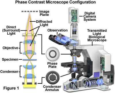
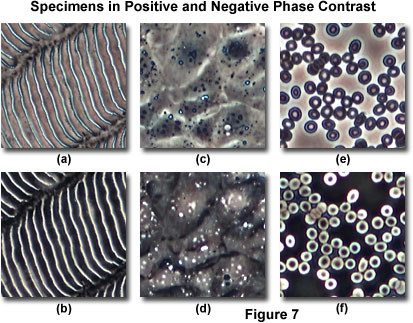
The phase contrast microscope
Ajusting the contrast
Rich ... but somewhat "qualitative"
A first step towards holography
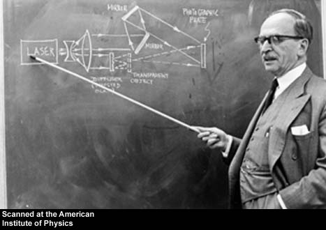
More than 3D
"known" (controled) reference wave
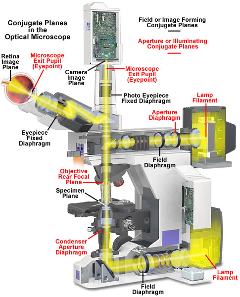
Stigmatism and the microscope

Points \(B\), \(B'\) and \(B''\) are conjugate points ; there is a bijective relation between them.
This is not the case in "real life" microscopy
Young's slits experiment
Interference pattern
Abbe's theory of image formation
$$ d=\frac{\lambda}{2n\sin \alpha}$$
An image is a spatial distribution of intensity, the intensity of the total field reaching the image plane
This total field can be expressed as the sum of individual fields and the image can "viewed" as the interference pattern genrated by these individual fileds !
Fourier series
Any periodic function \(f(t)\) of period \(T\) (pulsation \(\omega\), \(\omega T=2\pi\)) can be expressed as :
\begin{align*}
f(t) &= a_0 + a_1\sin\omega t + b_1 \cos\omega t + a_2\sin 2\omega t + b_2 \cos 2\omega t + \ldots \\\
&= a_0 + \sum_n a_n \sin n\omega t + \sum_n b_n \cos n\omega t
\end{align*}
Abbe's diffraction limit
Diffraction limit
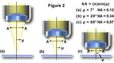
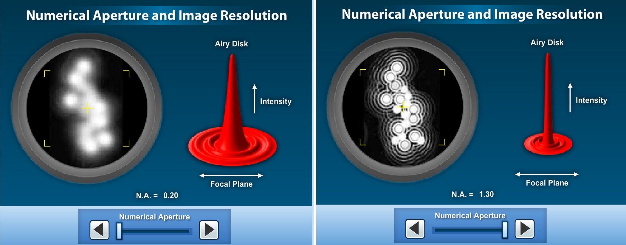
Numerical aperture
Numerical aperture
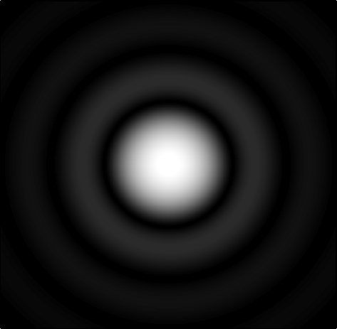
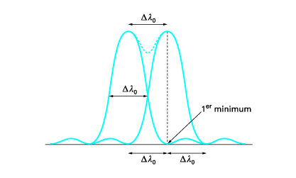
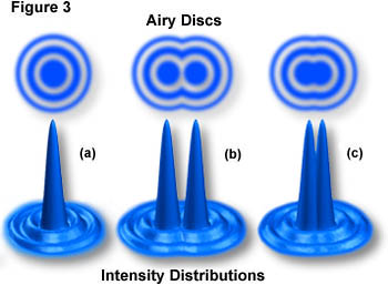
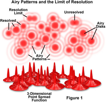
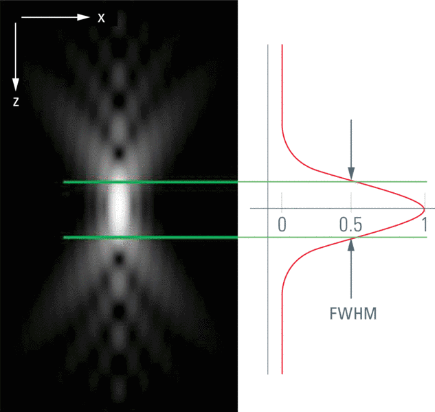
Airy pattern and Rayleigh criterion
 $$I(\theta) = I_0 \left ( \frac{2 J_1(ka \sin \theta)}{ka \sin \theta} \right )^2$$
$$k = \frac{2\pi}{NA}$$
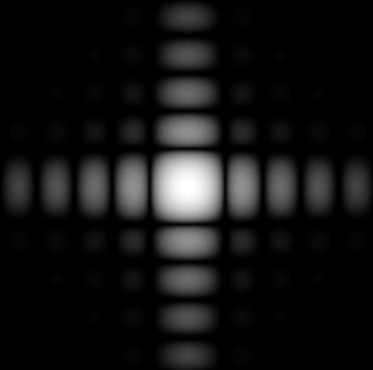
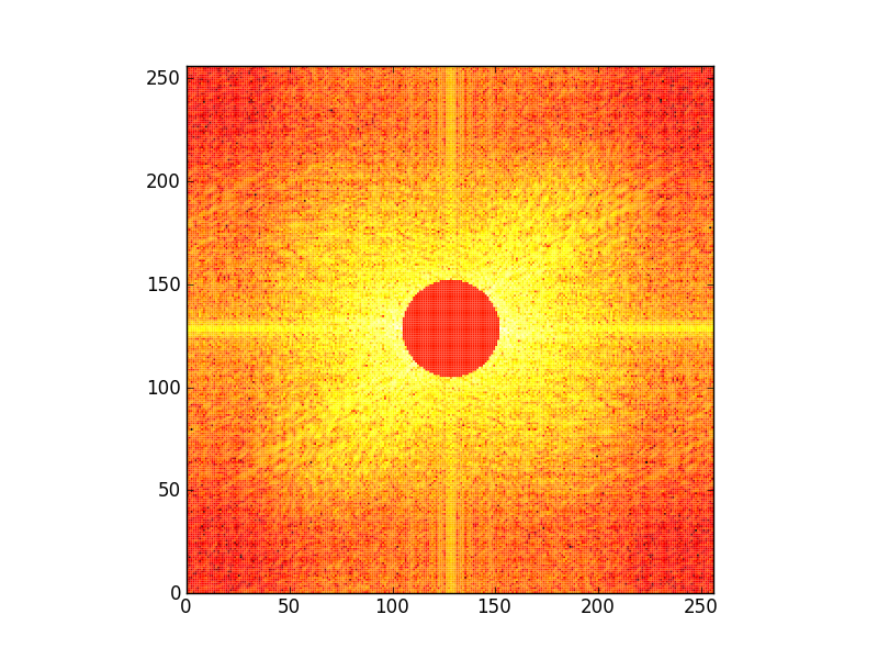
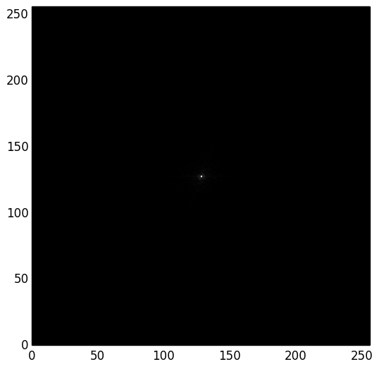
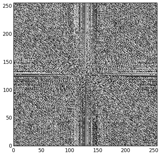
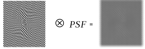
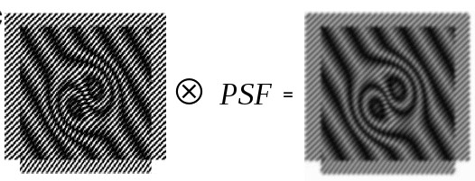
PSF and imaging
PSF, Impulse response ... Convolution
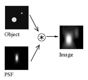
The imaging system (microscope) is linear invariant system analogous to a LTI : $$I(x,y)=PSF(x,y)*O(x,y)$$
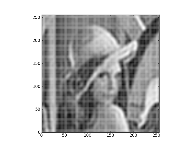
Deconvolution
Deconvolution is possible to a certain extent ...
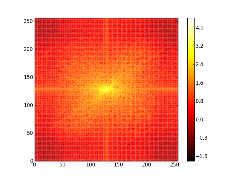
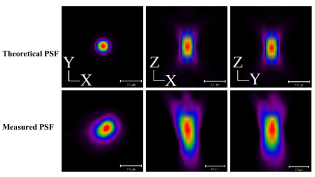
Real PSF
A 3D problem
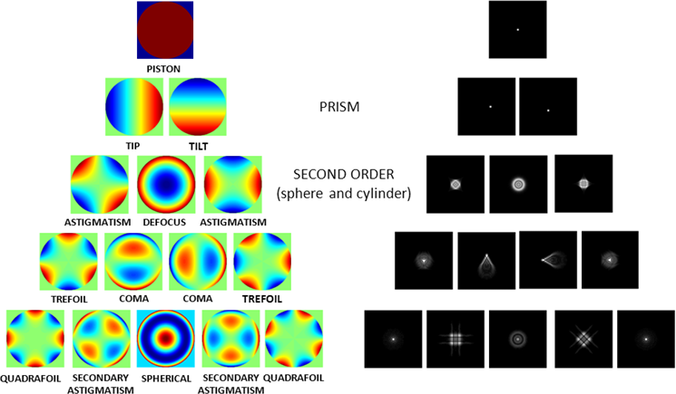
Aberrations
Optical element are not perfect.
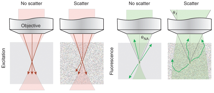
Scattering
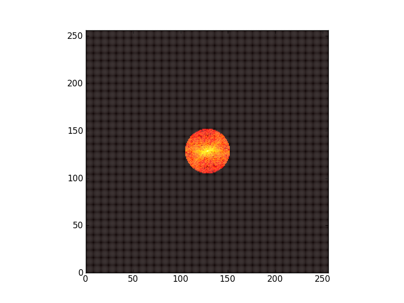
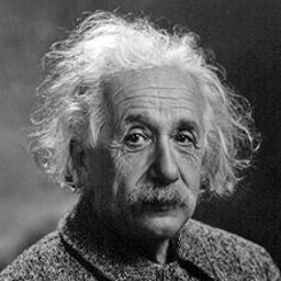
Measuring the PSF : Imaging a very small object
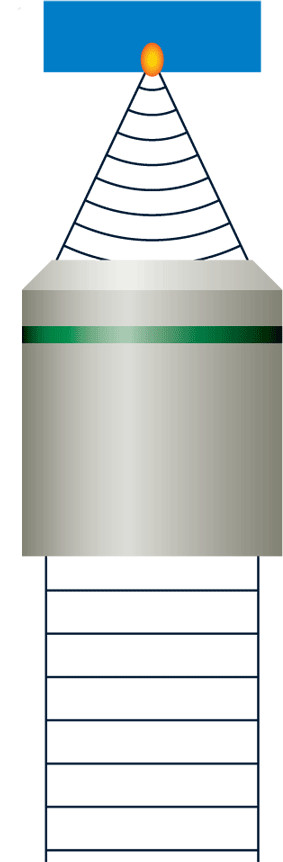
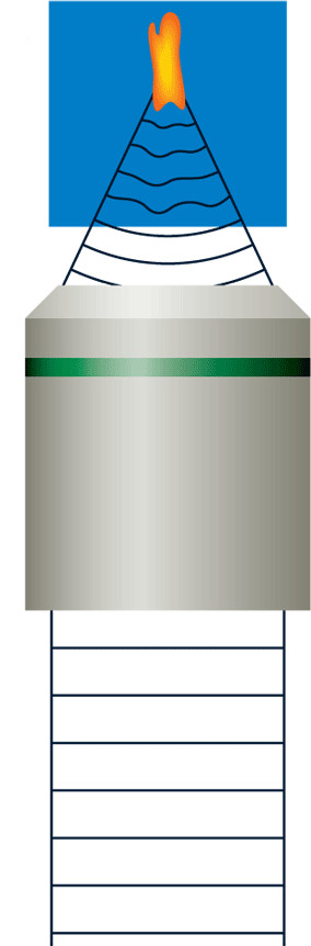
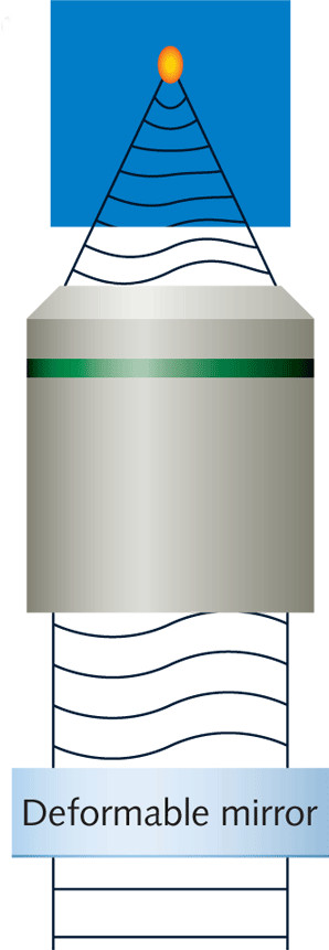
Improving the PSF with Adaptative Optics (AO)
Conclusion
- Determine the required PSF for your needs
- What is the smallest feature (x,y,z) you need to image ?
- What is the sample thickness
- Estimate the PSF of your system
- What is the NA of your objective ?
- Measure and if necessary improve the real PSF
- Image small, well separated, beads
- Consider Wavefront Engineering (call The Wavefront Engineering Group !) ...
- ... or superresolution techniques
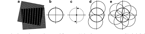
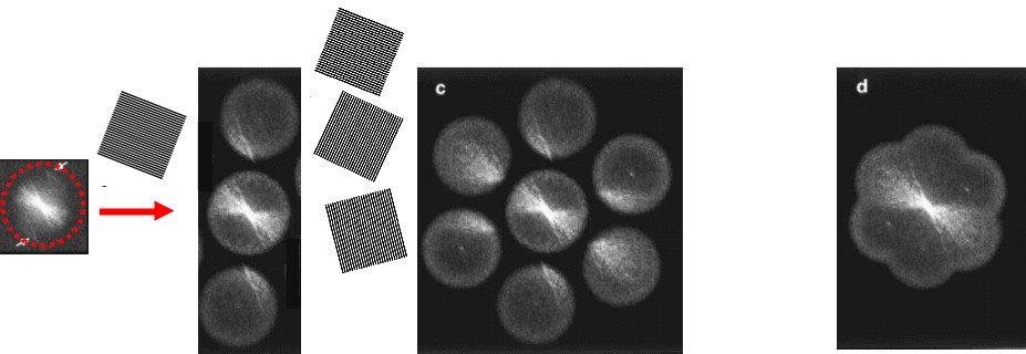
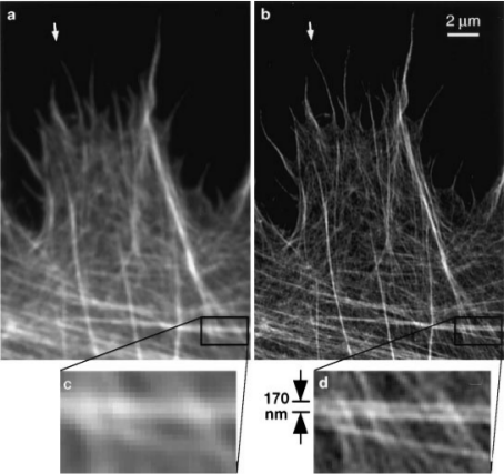
Illumination
structurée
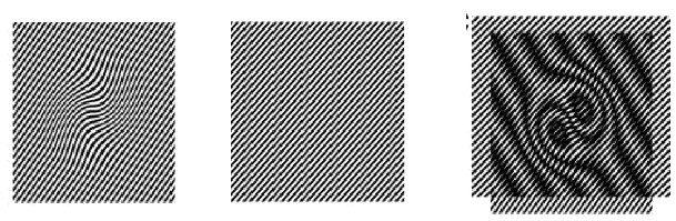
Moiré
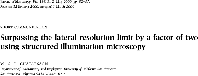
Modulation d'amplitude
En 1D :
$$\cos(2\pi f_0 x) \times \cos(2\pi f_1 x) = \frac{1}{2}\left[\cos(2\pi (f_1-f_0) x)+\cos(2\pi (f_1+f_0) x)\right]$$En 3D :

Microscopie HiLo
Emiliano Ronzitti
Résolution axiale
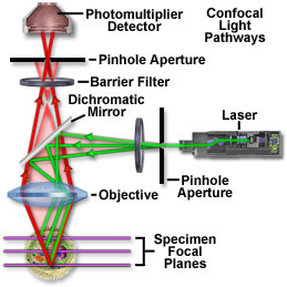
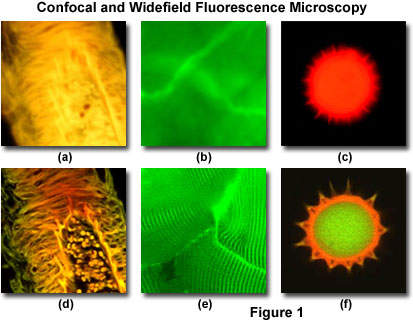
Microscopie confocale
The traveling wave
$$\tilde{E}=\tilde{A}e^{j( \omega t \pm kr)}$$For example, a sound wave : $$f=1000\,{\rm Hz} \; ;\; c=330\,{\rm m.s^{-1}} \quad\to\; \lambda = 0,33\,\textrm{m}$$
Propagating wave : the phasor
\begin{align} \omega t -kw &= \varphi_0 \\ x &= \frac{\varphi_0}{k}+\frac{\omega}{k}t \\ &= \frac{\varphi_0}{k}+ct \end{align}
One particular "point" of phase \(\varphi_0\) travels along the axis \(Ox\) at speed \(c\).
2D - 3D waves : the wavefront
In 2D (3D) a given path (surface) of same phase form a "wavefront"

The wave vector
The wave vector indicates the (local) direction of propagation of the wave.

For the "locally plane" wavefront : $$ \vec k\cdot \vec r = \rm{cst} $$
The wave vector is normal to the wave front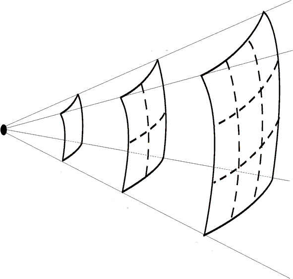
$$ \vec k\cdot \vec r = {\rm cst} \quad\to \quad \tilde{E}=\tilde{A}e^{j( \omega t \pm \vec k \cdot \vec r)}$$
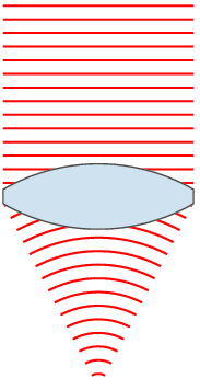
from wave optics back to ray optics
Snell's law : refraction
Diffrent thickness \(\to\) different phase shift (retardation).
$$ \Delta \varphi(x) = 2\pi (n-1) \frac{x \tan \alpha}{\lambda}$$
Axicon
lens
Wavefront engineering

Tilt
Lens
Multi spots
Wavefront Engineering
Diffractive Optical Elements (DOE)
For any point (x,y) of the incoming wavefront we want to add independantly the appropriate phase delay
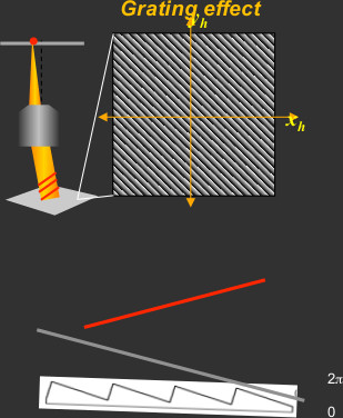 $$\Delta\phi_g=a\left(x\tan\theta_x+y\tan\theta_y\right)\textrm{mod }2\pi$$
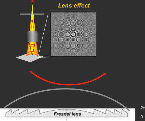 $$\phi_\ell=b\Delta z\left(x^2+y^2\right)\textrm{mod }2\pi$$
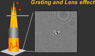 $$\phi=\textrm{arg }\left(\sum_1^N u_n e^{i\left(\phi_g+\phi_\ell\right)}\right)\textrm{mod }2\pi$$

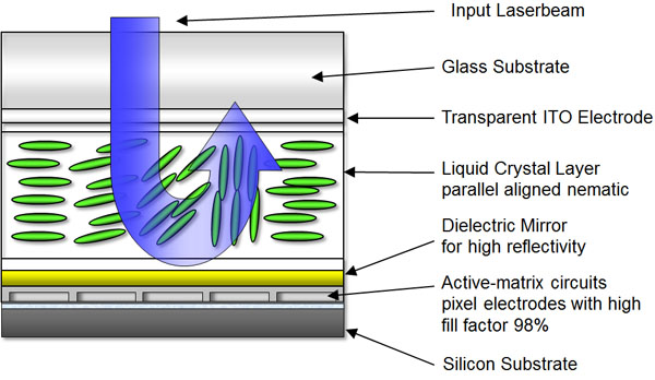
Liquid crystal spatial light modulator (SLM)
Conclusion
- Phase modulation in back focal plane can shape intensity in the focal plane
- Phase profiles can be calculated (to a pretty good approximation) for any shape
- SLMs are flexible and cool tools
- Fourier optics is your friend
Oscillateur harmonique
Considérons un système à l'équilibre que l'on déplace légèrement par rapport sa position d'équilibre L'énergie potentielle du système \(E_p\) pour cette nouvelle position \(x\) légèrement différente de celle d'équilibre \(x_{eq}\) s'écrit, après un développement limité à l'ordre 2 :
$$E_p(x) = E_p(x_{eq}) + (x-x_{eq})\left. \frac{dE_p}{dx}\right|_{x_{eq}} + \frac{(x-x_{eq})^2}{2}\left. \frac{d^2E_p}{dx^2}\right|_{x_{eq}} + O((x-x_{eq})^2)$$Par souci de simplicité on suppose que l'énergie \(E_p\) est fonction de la position \(x\) mais le raisonnement sera le même pour toute variable dont dépend l'énergie et que l'on aura modifiée.
- \(x_{eq}\) étant une position d'équilibre : \(\displaystyle \left. \frac{dE_p}{dx}\right|_{x_{eq}} = 0\)
- \(x_{eq}\) étant une position d'équilibre stable : \(\displaystyle \left. \frac{d^2E_p}{dx^2}\right|_{x_{eq}}\equiv k > 0\)
On peut donc écrire : $$ E_p(x) \approx E_p(x_{eq}) + \frac{1}{2}k(x-x_{eq})^2$$
On s'intéresse maintenant à la force de rappel (qui "ramène" le système vers sa position d'équilibre). A partir de la relation entre travail et énergie potentielle : $$ \vec F = - \vec\nabla E_p \quad\to\quad F_x(x)=-\frac{dE_p}{dx}$$
on obtient : $$ E_p(x) \approx E_p(x_{eq}) + \frac{1}{2}k(x-x_{eq})^2 \quad\to\quad F_x(x)=-k(x-x_{eq})$$
Au voisinage de \(x_{eq}\) le système se comporte comme un oscillateur harmonique si il est soumis à une force de rappel élastique
Oscillateur harmonique amorti
On considère maintenant une force de frottement proportionnelle (et de sens opposé) à la vitesse (Rappelez-vous la PACES ;-)) $$\vec F_f = - \gamma \frac{\partial x}{\partial t} \; ; \gamma > 0 $$ $$m\frac{\partial^2 x}{\partial t^2} + \gamma \frac{\partial x}{\partial t} + kx = 0 \quad\to\quad \frac{\partial^2 x}{\partial t^2} + \frac{1}{\tau} \frac{\partial x}{\partial t} + \omega_0^2x = 0 $$
- \(\displaystyle \omega_0=\sqrt{\frac{k}{m}}\) : résonance. \(\displaystyle [\omega_0]=\sqrt{\frac{[MT^{-1}]}{[M]}}=[T^{-1}]\)
- \(\displaystyle \tau = \frac{m}{\gamma}\) : temps caractéristique. \(\displaystyle [\tau]=\frac{[M]}{[MT^{-1}]}=[T]\)
- \(Q=\omega_0\tau\) : facteur de qualité. \([Q]=[T^{-1}T]=[]\)
- \(\displaystyle \zeta=\frac{1}{2Q} \) : facteur d'amortissement. \(\displaystyle [\zeta]= \frac{1}{[Q]}=[]\)
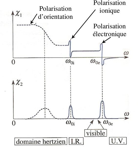
Polarisation induite
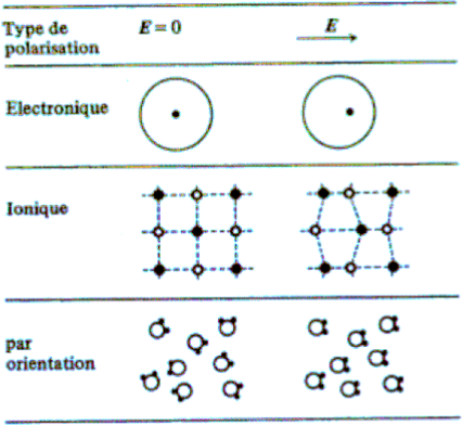
Il apparaît un champ induit \(\tilde{\vec P}\) proportionnel au champ appliqué \(\tilde {\vec E}\) (au moment dipolaire induit \(\tilde{\vec p}\))
- \(\chi_e\) : susceptibilité électrique
Vecteur déplacement :
\begin{align} \tilde{\vec D} &= \epsilon_0 \tilde{\vec E} +\tilde{\vec P}\\ &= \epsilon_0 \underbrace{\left(1+\chi_e\right)}_{\epsilon_r\,\textrm{perm. rel.}}\tilde{\vec E} \end{align}Modèle de l'électron élastiquement lié
La force appliquée à l'oscillateur harmonique amorti s'écrit :
$$ q\tilde{E}=q\tilde{E_0}e^{j\omega t}$$
$$\tilde{\vec x} = \frac{\frac{q}{m\omega_0}}{1+j\frac{1}{Q}\frac{\omega}{\omega_0}-\frac{\omega^2}{\omega_0^2}} \tilde{E_0}$$
$$\tilde{\vec p} = q\tilde{\vec x} $$
$$\tilde\chi_e= \frac{\chi_0}{1+j\frac{1}{Q}\frac{\omega}{\omega_0}-\frac{\omega^2}{\omega_0^2}} \qquad \chi_0\equiv\chi_e(\omega=0)= n^*\frac{q^2}{m\epsilon_0\omega_0^2}$$
LA susceptibilité est une quantité complexe, on pose \(\tilde\chi_e = \chi_1-j\chi_2\) :
$$\chi_1=\frac{1-\frac{\omega^2}{\omega_0^2}}{\left(1-\frac{\omega^2}{\omega_0^2}\right)^2+\left(\frac{1}{Q}\frac{\omega}{\omega_0}\right)^2}\chi_0 \qquad \chi_2=\frac{\frac{1}{Q}\frac{\omega}{\omega_0}}{\left(1-\frac{\omega^2}{\omega_0^2}\right)^2+\left(\frac{1}{Q}\frac{\omega}{\omega_0}\right)^2}\chi_0 $$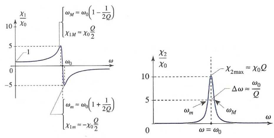
Ici \(Q=10\), en réalité \(Q\) est de l'ordre de \(10^3\)à \(10^4\)
Retour aux ondes EM
 \begin{align}
\vec \nabla \cdot \vec D &= \rho \\
\vec \nabla \cdot \vec B &= 0 \\
\vec \nabla \times \vec E &= -\frac{\partial\vec B}{\partial t} \\
\vec \nabla \times \vec B &= \mu_0 \vec j + \mu_0\frac{\partial\vec D}{\partial t} \\
\end{align}
\begin{align}
\vec \nabla \cdot \vec D &= \rho \\
\vec \nabla \cdot \vec B &= 0 \\
\vec \nabla \times \vec E &= -\frac{\partial\vec B}{\partial t} \\
\vec \nabla \times \vec B &= \mu_0 \vec j + \mu_0\frac{\partial\vec D}{\partial t} \\
\end{align}
$$\vec D = \epsilon_0\epsilon_r \vec E$$
Dans un milieux "sans charges libres ni courant" : \( \rho\,,\,\vec j = 0\)
 $$-\nabla^2 \vec E +\frac{\epsilon_r}{c^2} \frac{\partial^2 \vec E}{\partial t^2} = 0$$
$$ c=\frac{1}{\sqrt{\mu_0\varepsilon_0}} $$
$$-\nabla^2 \vec E +\frac{\epsilon_r}{c^2} \frac{\partial^2 \vec E}{\partial t^2} = 0$$
$$ c=\frac{1}{\sqrt{\mu_0\varepsilon_0}} $$
\(c\) est la célérité dans le vide, \(c/\sqrt{\epsilon_r}\) la vitesse dans le milieu
Indice de réfraction
L'indice de réfraction est une quantité complexe !
$$ \tilde n^2 = \tilde\epsilon_r = 1 + \tilde\chi_e$$En général \(|\chi_e| << 1\) :
$$ \tilde n \approx 1 +\frac{\chi_e}{2} \quad\to\quad n_1-jn_2 = 1+\frac{\chi_1}{2}-j\frac{\chi_2}{2}$$Équation de d'Alembert :
solutions harmoniques
$$\frac{\partial^2 \tilde E}{\partial x^2} - \frac{1}{\left(c/\tilde n\right)^2}\frac{\partial^2 \tilde E}{\partial t^2}=0 $$
$$\tilde E= \tilde{E_0} e^{j(\omega t -\tilde k x)}$$
Loi de Beer-Lambert
$$\tilde E = \tilde E_0 \exp\left(j\left(\omega t -\frac{2\pi}{\lambda}n_1x+j\frac{2\pi}{\lambda}n_2x\right)\right)$$